import datetime
import geospacelab.datahub as datahub
import geospacelab.visualization.mpl as gsl_mpl
Swarm Data Access
Initial settings
dt_fr = datetime.datetime(2016, 3, 15, 18, 18)
dt_to = datetime.datetime(2016, 3, 15, 18, 23)
sat_id = "A"
Create a datahub
dh = datahub.DataHub(dt_fr=dt_fr, dt_to=dt_to, visual='on')Dock a Swarm dataset
Docking a dataset is the process of loading the dataset into the datahub. It is done by calling the dock method of the datahub object. The method takes the name patterns of the dataset as an argument and returns a dataset object.
The following code docks the Swarm MAG LR dataset for the specified time range (shown above) and satellite ID. A full list of the supported datasets and their name patterns can be found in the Supported datasets tutorial.
ds = dh.dock(datasource_contents=['esa_eo', 'swarm', 'l1b', 'mag_lr'], sat_id=sat_id, add_APEX=True,)Load IGRF coefficients ...
Searching the data product "MAG_LR" with the version "latest" on the server...
The file [PosixPath('/data/afys-ionosphere/data/ESA/SWARM/Level1b/MAG_LR/0701/Sat_A/2016/SW_OPER_MAGA_LR_1B_20160315T000000_20160315T235959_0701_MDR_MAG_LR.cdf'), PosixPath('/data/afys-ionosphere/data/ESA/SWARM/Level1b/MAG_LR/0701/Sat_A/2016/SW_OPER_MAGA_LR_1B_20160315T000000_20160315T235959_0701_ASM_VFM_IC.cdf')] already exists: skip downloading.
WARNING: Multiple files found for the pattern *20160315T000000*20160315T235959*0701*.cdf in the directory /data/afys-ionosphere/data/ESA/SWARM/Level1b/MAG_LR/0701/Sat_A/2016!
/opt/anaconda3/envs/Swarm/lib/python3.12/site-packages/numpy/_core/numeric.py:476: RuntimeWarning: invalid value encountered in cast
  multiarray.copyto(res, fill_value, casting='unsafe')
List the variables included in the dataset
ds.list_all_variables()Dataset: esa/earthonline | swarm | mag | mag_lr
Printing all of the variables ...
|No. |Variable name |Variable name (Source) |Description |
|--------------------|------------------------------|------------------------------|----------------------------------------------------------------------------------------------------|
|1 |SC_DATETIME |N/A |Time of observation |
|2 |SYNC_STATUS |SyncStatus | |
|3 |SC_GEO_LAT |Latitude |Geographic Latitude |
|4 |SC_GEO_LON |Longitude |Geographic Longitude |
|5 |SC_GEO_r |N/A | |
|6 |B_VFM |B_VFM | |
|7 |B_VFM_x |N/A |B in x direction of VFM frame |
|8 |B_VFM_y |N/A |B in y direction of VFM frame |
|9 |B_VFM_z |N/A |B in z direction of VFM frame |
|10 |B_VFM_x_err |N/A | |
|11 |B_VFM_y_err |N/A | |
|12 |B_VFM_z_err |N/A | |
|13 |B_NEC |B_NEC | |
|14 |B_N |N/A |B in northward direction of NEC frame |
|15 |B_E |N/A |B in eastward direction of NEC frame |
|16 |B_C |N/A |B in downward direction of NEC frame |
|17 |dB_Sun_VFM |dB_Sun | |
|18 |dB_Sun_VFM_x |N/A |dB due to Sun induced perturbation in x direction of VFM frame |
|19 |dB_Sun_VFM_y |N/A |dB due to Sun induced perturbation in y direction of VFM frame |
|20 |dB_Sun_VFM_z |N/A |dB due to Sun induced perturbation in z direction of VFM frame |
|21 |dB_AOCS_VFM |dB_AOCS | |
|22 |dB_AOCS_VFM_x |N/A |dB due to AOCS induced perturbation in x direction of VFM frame |
|23 |dB_AOCS_VFM_y |N/A |dB due to AOCS induced perturbation in y direction of VFM frame |
|24 |dB_AOCS_VFM_z |N/A |dB due to AOCS induced perturbation in z direction of VFM frame |
|25 |dB_other_VFM |dB_other | |
|26 |dB_other_VFM_x |N/A |dB due to all other sources of perturbation in x direction of VFM frame |
|27 |dB_other_VFM_y |N/A |dB due to all other sources of perturbation in y direction of VFM frame |
|28 |dB_other_VFM_z |N/A |dB due to all other sources of perturbation in z direction of VFM frame |
|29 |B_VFM_err |B_error | |
|30 |q_NEC_CRF |q_NEC_CRF | |
|31 |Att_error |Att_error | |
|32 |FLAG_B |Flags_B |Flag B |
|33 |FLAG_q |Flags_q |Flag q |
|34 |FLAG_Platform |Flags_Platform |Flag Platform |
|35 |FLAG_B_BIN_AUX |N/A |Binary flag for B |
|36 |FLAG_B_BIN_IND |N/A | |
|37 |FLAG_q_BIN_AUX |N/A |Binary flag for q |
|38 |FLAG_q_BIN_IND |N/A | |
|39 |FLAG_Platform_BIN_AUX |N/A |Binary flag for Platform |
|40 |FLAG_Platform_BIN_IND |N/A | |
|41 |FLAG_F |Flags_F |Flag F |
|42 |FLAG_F_BIN_AUX |N/A |Binary flag for F |
|43 |FLAG_F_BIN_IND |N/A | |
|44 |ASM_Freq_Dev |ASM_Freq_Dev | |
|45 |F |F |Magnetic field intensity |
|46 |F_err |F_error | |
|47 |dF_Sun |dF_Sun | |
|48 |dF_AOCS |dF_AOCS | |
|49 |dF_other |dF_other | |
|50 |SC_APEX_LAT |N/A |APEX Latitude |
|51 |SC_APEX_LON |N/A |APEX Longitude |
|52 |SC_APEX_MLT |N/A |APEX Magnetic Local Time |
|53 |SC_GEO_LST |N/A |Local Solar Time |
Get a variable and data array
B_N = ds['B_N']This returns a GeospaceLAB Variable object, which contains the data array and its metadata. The data array is a NumPy array, which can be used for further analysis and calculations. The metadata includes the variable name, full name or description, unit, and other attributes. The variable object also has built-in visual attributes and methods for plotting and visualizing the data. See more details in Visualization.
To get the data array, call
B_N_arr = B_N.valueAbove returns a numpy.ndarray data array.
Swarm Data Visualization
The following example shows how to make the time series plots in GeospaceLAB with the Swarm MAG LR data. More examples can be found in Examples
# Create a figure
fig = gsl_mpl.create_figure(figsize=(8, 12))
# Add a time series dashboard to the figure
db = gsl_mpl.dashboards.TSDashboard(figure=fig, dt_fr=dt_fr, dt_to=dt_to)
# Set the panel layouts in the dashboard.
# The layout is a list of lists, where each inner list represents a row of panels in the dashboard.
# Each element in the inner list is a variable from the dataset that will be plotted in that panel.
# This allows for flexible arrangement of multiple plots in a single dashboard.
# To add or remove a panel, simply modify the inner lists accordingly.
# For example, to remove the first panel, simply remove the first inner list: panel_layouts = [ [ds['B_N'], ds['B_E'], ds['B_C']], ... ]
panel_layouts = [
    [ds['F']],
    [ds['B_N'], ds['B_E'], ds['B_C']],
    [ds['B_VFM_x'], ds['B_VFM_y'], ds['B_VFM_z']],
    [ds['dB_Sun_VFM_x'], ds['dB_Sun_VFM_y'], ds['dB_Sun_VFM_z']],
    [ds['dB_AOCS_VFM_x'], ds['dB_AOCS_VFM_y'], ds['dB_AOCS_VFM_z']],
    [ds['dB_other_VFM_x'], ds['dB_other_VFM_y'], ds['dB_other_VFM_z']],
    [ds['FLAG_F_BIN_AUX']],
    [ds['FLAG_B_BIN_AUX']],
    [ds['FLAG_q_BIN_AUX']],
    [ds['FLAG_Platform_BIN_AUX']],
]
db.set_layout(panel_layouts)
# Plotting the data in the dashboard
db.draw()
# Add panel labels to the dashboard
db.add_panel_labels()
# Add a title to the dashboard
db.add_title(y=1.02,title='Swarm-{} MAG LR Zoom'.format(ds.sat_id), fontsize='medium', append_time=True)
# Show the figure/dashboard
db.show() 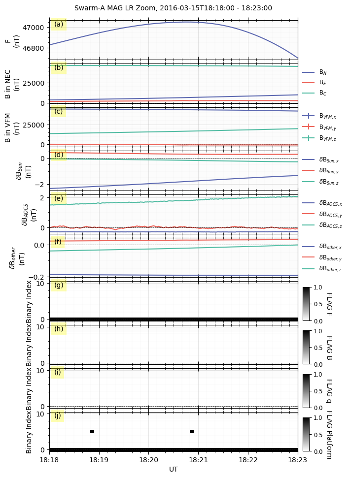
As shown in the figure, the Swarm MAG LR data can be visualized in GeospaceLAB with the same functions as other datasets. The unified interface allows users to easily switch between different data products and visualize them seamlessly. The data from different satellites can be plotted together for comparison. The plot can be customized with various options, such as color, line style, and markers. The plot can also be saved in various formats, such as PNG, PDF, and SVG. See more details in Visualization.